Build Defensible Parametric CERs in 6 Steps for Construction

Parametric estimating uses statistical relationships between cost and measurable project attributes, like square footage, tonnage, or capacity, to generate a cost figure without a full quantity takeoff. It works best in early feasibility and concept design, when the design has enough definition to identify real cost drivers but not enough detail for a line-item estimate. Accuracy depends entirely on the quality of the historical data behind the model, and it is not a substitute for a detailed estimate once the design solidifies.

TL;DR:

• Parametric estimating is most effective early in design, relying on quality historical data, and less accurate when new technologies or limited data are involved.
• Building a reliable CER requires normalizing data for time, location, and scope, and documenting all assumptions and judgment calls explicitly.
• Regression analysis with appropriate functional forms and validation metrics ensures the statistical robustness of the cost model, especially when using multiple variables.
• Regular calibration, validation, and sensitivity analysis are essential to maintain model accuracy and provide meaningful uncertainty ranges for stakeholders.
• Using platforms like ArosBid streamlines data collection and normalization, improving model reliability and reducing setup time for project estimates.

Table of Contents

• What Is Parametric Estimating in Construction?
• The Parametric Estimating Process, Step by Step
• Building CERs: Regression Methods and Model Fit
• Calibration, Validation, and Sensitivity Analysis
• How Accurate Is Parametric Estimating? Estimate Classes Explained
• Worked Examples: A Simple Formula and a Multi-Variable Model
• Tools, Data Sources, and Shortcuts That Actually Save Time
• How ArosBid Complements Parametric Estimating in Real Bid Workflows
• What Experienced Estimators Get Right (And Where Most Models Fail)
• Turn Parametric Data Into Better Bids With ArosBid
• Sources
• FAQ

What Is Parametric Estimating in Construction?

Construction professionals typically choose from four estimating methods, and each one fits a different stage of a project’s life. Parametric estimating sits in a specific spot on that spectrum, and knowing where helps you avoid using the wrong tool for the job.

Unit cost estimating prices individual line items, like cost per linear foot of duct or per cubic yard of concrete, and demands a fairly developed design. Assembly estimating groups related components (a wall assembly, a roof system) into a single composite rate, useful once you have schematic drawings. Analogous estimating leans on a single comparable past project and scales it by judgment more than math. Parametric estimating differs from all three because it builds a statistical model, a cost estimating relationship (CER), from multiple historical data points rather than one comparable job or a full component list.

RSMeans frames the four methods as sitting along a continuum of design maturity, with parametric estimating occupying the early to mid-design window where a handful of technical or programmatic attributes correlate strongly with cost. A hospital’s cost might correlate well with bed count and square footage. A warehouse’s cost might scale predictably with clear height and dock door count. If that relationship holds across a reasonable data set, you have a candidate for a parametric model.

Parametric estimating earns its keep at specific project stages:

• Feasibility studies, where owners need a rough budget before committing to design fees
• Concept and schematic design, when scope is defined enough to identify drivers but drawings are not complete
• Portfolio-level planning, where dozens of similar projects need consistent, comparable budgets
• Value engineering exercises, where you need to test the cost impact of changing a single variable quickly

Parametric estimating breaks down in a few predictable situations. If the project uses a genuinely novel technology or construction method, no historical database exists to build a CER from. If you are pricing a final bid, subcontractors need quantities and unit prices, not a statistical approximation. And if your historical data set is thin, say, fewer than eight or ten comparable projects, the regression behind the model has little statistical power, no matter how clean the math looks. RSMeans notes that parametric estimating trades some precision for speed and objectivity, which is exactly the trade you want early, and exactly the trade you cannot afford at the guaranteed maximum price stage.

The Parametric Estimating Process, Step by Step

Building a parametric model is not a single calculation. It is a sequence of decisions, and skipping one usually shows up later as an estimate nobody trusts. The ICEAA Parametric Estimating Handbook frames this as a database-first discipline: the model is only as good as what feeds it, and that framing should guide every step below.

1. Define scope and pick a cost basis. Decide up front whether you are estimating total installed cost (TIC), hard construction cost only, or a cost-per-square-foot figure. Mixing bases across your historical data set is one of the fastest ways to produce a meaningless regression.
2. Identify candidate cost drivers. Brainstorm every measurable attribute that plausibly correlates with cost: square footage, tonnage, HVAC tonnage, number of fixtures, linear feet of piping, occupancy type. Then separate true drivers from passengers, variables that move with cost by coincidence rather than causation. A driver has a defensible physical or programmatic link to cost; a passenger just happens to correlate in your sample.
3. Collect historical data and record metadata. Pull cost data from completed projects, and for each one, log the year, location, and scope description alongside the cost figure. Without that metadata, you cannot normalize the data in the next step, and an unnormalized data set produces a CER that looks precise and is actually wrong.
4. Normalize for time, location, and scope. Inflate or deflate every historical cost to a common cost year, apply location factors to account for regional labor and material differences, and adjust for scope differences like site conditions or finish level. The ICEAA handbook is explicit that normalization has to account for inflation, location, scope, productivity assumptions, and nonrecurring costs, because skipping any one of these yields a regression coefficient that is technically calculated but practically meaningless.
5. Select a single-driver CER or a multi-variable regression. If one variable explains most of the cost variance, a simple CER, cost as a function of that one driver, is often sufficient and easier to defend. If cost depends on several interacting factors (square footage, occupancy type, and mechanical system complexity, for instance), you need multi-variable regression, and you need to watch for the statistical pitfalls covered in the next section.
6. Document assumptions and keep an audit trail. Every normalization factor, every excluded data point, and every judgment call about scope needs to be written down. When someone questions the estimate six months later, and someone will, your audit trail is what turns “trust me” into “here’s exactly how I got this number.”

Pro Tip: Keep a running log of every project you exclude from your data set and why. Reviewers almost never question the data you included. They question the data you left out, and if you can’t explain that decision on the spot, the whole model loses credibility.

Estimators who build this workflow into a repeatable checklist, rather than reinventing it project by project, end up with faster turnaround and fewer surprises when a model gets audited. That repeatability is also why your data collection habits matter more than any single regression run. Vendor quotes and actuals captured cleanly during bidding, rather than reconstructed later from memory or scattered spreadsheets, are what make step three fast instead of painful. A platform like ArosBid’s bid management system that already logs quote data in a structured format gives you a running head start on this exact step.

Building CERs: Regression Methods and Model Fit

A cost estimating relationship is only as good as the math behind it, and that math starts with picking the right functional form. Linear CERs (cost = a + b × driver) work when cost increases at a constant rate as the driver increases. Power CERs (cost = a × driver^b) fit situations with economies or diseconomies of scale, common in process industries where unit cost drops as capacity grows. Log-linear forms show up when the driver’s effect on cost is multiplicative rather than additive. Getting this choice wrong doesn’t just hurt accuracy, it can make your coefficients uninterpretable, so plot your data before you regress anything. If the scatter curves, a straight line will lie to you no matter how good the fit statistics look.

Regression analysis, specifically Ordinary Least Squares (OLS), is the standard method the industry uses to derive CERs, fitting a line or curve that minimizes the squared distance between predicted and actual costs. OLS works cleanly for single-driver models. Multi-variable regression, where cost depends on two or more drivers simultaneously, introduces a real hazard: multicollinearity, where two independent variables are themselves correlated with each other. If square footage and number of floors both go into your model and they move together in your data set, the regression can’t cleanly separate their individual effects, and your coefficients become unstable.

Once you have a fitted model, the slope tells you the marginal cost per unit of driver, cost per additional square foot, cost per additional ton of HVAC capacity, and the intercept represents a fixed cost baseline independent of the driver. A negative or nonsensical intercept is often a sign your data range doesn’t extend low enough to trust extrapolation near zero.

Reporting model quality means presenting the diagnostics, not just the equation:

• R² (coefficient of determination): the share of cost variance the model explains; higher is better, but a suspiciously high R² on a small sample often signals overfitting rather than a genuinely strong relationship.
• Standard error (SE): how far actual costs typically deviate from the model’s prediction, in the same units as cost.
• t-test on each coefficient: confirms whether a given driver’s effect on cost is statistically distinguishable from zero.
• F-test on the overall model: confirms the regression as a whole explains more variance than chance would predict.
• Residual plots: a quick visual check for patterns in the errors, which would suggest the functional form is wrong even if R² looks acceptable.

By the Numbers: RSMeans recommends that defensible parametric estimates include statistical validation metrics like R², t-tests, and F-tests, paired with a documented audit trail of every normalization decision. A model without that reporting is an opinion with a formula attached.

Calibration, Validation, and Sensitivity Analysis

A model that fits your historical data well isn’t automatically trustworthy going forward. Calibration and validation are what separate a defensible CER from a curve-fitting exercise, and skipping them is how estimators end up defending a number they can’t actually explain.

Calibration means adjusting your model’s intercept or slope using the most recent actual project costs, so the CER reflects current market conditions rather than a data set that might be several years old. That’s a calibration signal telling you to shift the intercept before you trust the next output.

Validation techniques confirm the model generalizes beyond the data used to build it:

• Holdout sets: set aside a portion of your historical projects before fitting the model, then test predictions against those excluded projects.
• Cross-validation: repeatedly refit the model on different subsets of the data to check whether the coefficients stay stable across samples.
• Residual analysis: on the holdout set specifically, checking whether errors cluster in a way that suggests a missing variable.

NASA’s cost estimating handbook recommends holdout and prediction-set testing paired with residual analysis, noting that cross-validation is particularly important with small historical data sets, which describes most construction niches outside of high-volume repeatable building types.

Sensitivity analysis answers a different question: given the model you’ve validated, which variables actually move the needle? Practitioners run scenario-based sensitivity analysis to rank cost drivers by their influence on total cost, which then tells you where to spend your limited data-collection time and where design teams should focus value-engineering effort.

When you present results to stakeholders, show the range and the assumptions behind it, not just a single number. A budget of “$14.2 million” invites false confidence. A budget of “$13.1 million to $15.6 million, driven primarily by mechanical system capacity, based on twelve comparable projects normalized to current-year costs” invites an informed conversation.

Fall back to a bottoms-up estimate for that project and treat the parametric number as a sanity check instead of the answer.*

How Accurate Is Parametric Estimating? Estimate Classes Explained

Parametric estimating typically maps to AACE Class 4 or Class 5 estimates, the earliest, least design-developed categories in the AACE 18R-97 classification system. That’s not a weakness of the method. It’s the whole point: parametric models exist to give you a usable number before design has advanced far enough to support a detailed takeoff.

Class 4 conceptual estimates, the range where most parametric construction estimates live, commonly carry accuracy bands of roughly negative 30% to positive 50%, narrowing considerably as design progresses toward Class 3 and Class 2. That’s a wide range, and it should stay wide until the design gives you a reason to tighten it. Presenting a Class 4 parametric estimate as if it carries Class 2 precision is the single most common way estimators lose credibility with owners.

Estimate class should drive your contingency recommendation, not the other way around:

• Class 5 (conceptual screening): widest accuracy range, highest contingency, typically used for feasibility go/no-go decisions.
• Class 4 (concept/schematic): the parametric sweet spot, still wide accuracy bands, contingency set accordingly high.
• Class 3 (design development): accuracy tightens as quantities firm up, parametric methods start giving way to assembly and unit cost approaches.

Before you hand over any parametric figure, run through a short checklist: state the range, not a point number; list the top three drivers behind the figure; disclose the size and age of the data set behind the model; and flag any known scope items the model doesn’t capture.

Worked Examples: A Simple Formula and a Multi-Variable Model

The simplest parametric estimate scales a known historical cost by the ratio of a single parameter. The formula looks like this:

E_new = (C_old ÷ P_old) × P_new

Where C_old is a completed project’s actual cost, P_old is that project’s value for the driver (square footage, tonnage, whatever you’ve chosen), and P_new is the driver value for your current project. This scaling approach is a standard entry point into parametric estimating, and it works well for quick, low-stakes comparisons.

1. Say a completed 40,000 square foot warehouse cost $6,000,000 to build, or $150 per square foot.
2. Your new project is a similar warehouse at 55,000 square feet.
3. E_new = $150/SF × 55,000 SF = $8,250,000.

That’s a legitimate parametric estimate, and it took thirty seconds. It also assumes the two warehouses share clear height, dock configuration, and site conditions closely enough that a single driver captures the cost relationship. This is a real assumption worth stating out loud.

Once a second or third variable meaningfully affects cost, you need a multi-variable CER instead of a single ratio. A sketch might look like:

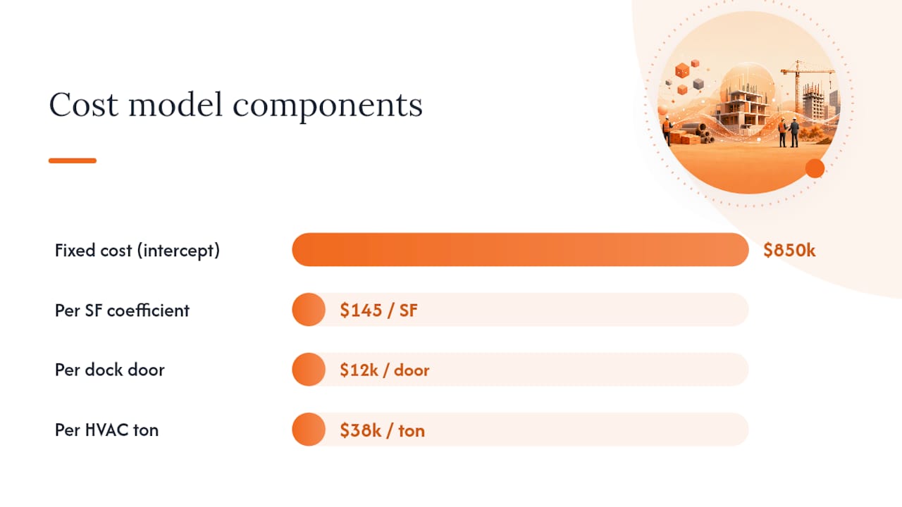
Cost = 850,000 + (145 × SF) + (12,000 × dock doors) + (38,000 × HVAC tons)

Here, the intercept ($850,000) represents fixed site and mobilization costs independent of size, and each coefficient represents the marginal cost contribution of that driver, holding the others constant. Reading this model correctly means checking that units line up (square feet, count of doors, tons of capacity) and that none of the three drivers are so correlated with each other that the coefficients become unstable, the multicollinearity issue covered earlier. The switch point from single formula to integrated multi-variable model usually arrives the moment a client or reviewer asks “what if we add two more dock doors?” and you realize a single $/SF number can’t answer that question.

Tools, Data Sources, and Shortcuts That Actually Save Time

RSMeans data (published under Gordian) remains one of the most widely referenced sources for unit costs and location factors, and it’s a reasonable starting point when your own historical data set is too thin to support a standalone CER. Cross-referencing an internal model against a published benchmark is a smart sanity check even when you have good proprietary data, because it catches the case where your own data set happens to be an outlier.

Spreadsheets handle a huge share of real-world parametric work, and there’s no shame in that. Excel with a solid regression add-in is entirely sufficient for single-driver and simple multi-variable CERs, especially when the audit trail matters as much as the math. Dedicated statistical software or purpose-built parametric platforms earn their cost when you’re running dozens of CERs across a portfolio, need automated sensitivity analysis across many variables at once, or require version control on a model that multiple estimators touch.

A few shortcuts are worth building into your standard workflow:

• Maintain normalized unit cost libraries by trade so you’re not renormalizing the same historical projects every time a new estimate comes up.
• Apply consistent location factors across your whole data set rather than picking them project by project, which introduces hidden inconsistency.
• Use quality multipliers (finish level, code requirements, site complexity) as adjustment factors rather than folding them invisibly into your base driver.

Be careful about vendor lock. Any platform, cost database, or proprietary CER library that doesn’t let you export the underlying data and see the calculation logic makes your estimates harder to audit later, and auditability is exactly what a defensible parametric model depends on.

How ArosBid Complements Parametric Estimating in Real Bid Workflows

Every parametric model lives or dies on its historical database, and that database is usually the weakest link in a busy estimating team’s process. Vendor quotes get scattered across email threads, Excel versions multiply, and by the time a project closes out, half the useful cost data never makes it into a usable format.

ArosBid’s bid command center captures and levels vendor quotes as they come in, which means the same data you’re already collecting to win a bid becomes the normalized historical record your next CER needs. A few specifics on how that plays out:

• Automated quote leveling standardizes scope and pricing format across vendors, cutting the normalization work described earlier in this guide down to a fraction of the effort.
• Actuals captured through the platform feed directly into calibration cycles, so your intercept and slope adjustments reflect current market data instead of a three-year-old spreadsheet.
• Integration with Excel and Outlook means estimators keep working in familiar tools while the underlying data structure stays clean enough for regression work later.
• Trade-specific workflows for steel, electrical, and mechanical scopes mean cost drivers particular to each trade, tonnage, load factors, equipment capacity, get captured consistently rather than reconstructed from memory after the fact.

The result isn’t a replacement for the statistical work covered in this guide. It’s a cleaner input to it.

What Experienced Estimators Get Right (And Where Most Models Fail)

Good parametric estimating comes down to discipline most teams skip under deadline pressure: validate your data before you trust it, normalize every figure for time, location, and scope, and write down every assumption as you make it, not after someone asks.

The mistakes we see repeatedly: building a model on unvalidated or unnormalized data, chasing a high R² on a tiny sample until the model overfits, ignoring scope drift between the historical projects and the current one, skipping normalization because “the projects are close enough,” and handing a stakeholder a single number instead of a range with drivers attached.

Pro Tip: When your data set has fewer than eight comparable projects, or when the current project involves a genuinely new system type, stop trying to force a parametric model. A bottoms-up, component-level estimate will serve you better than a regression with no real statistical power behind it.

— arosbid team

Turn Parametric Data Into Better Bids With ArosBid

Every parametric model needs cleaner, faster access to real project data than most estimating teams currently have, and that’s the exact gap this solution closes. Instead of chasing vendor quotes across email threads and rebuilding spreadsheets every time a bid closes out, a command center captures and levels quotes automatically, giving you a normalized, audit-ready data set that feeds directly into your next CER.

That matters most in the two places parametric estimating tends to break down: data quality and calibration. Instead of manually normalizing historical costs project by project, teams using ArosBid pull leveled, structured actuals straight from completed bids, which cuts the setup time behind sensitivity analysis and scenario runs dramatically. Whether you’re managing steel, electrical, or mechanical scopes, the platform’s industry-specific workflows mean the drivers that matter to your trade get captured consistently instead of reconstructed from memory months later. If your last estimate review turned into a debate about where the numbers came from, book a live demo and see how a cleaner data pipeline changes that conversation.

Sources

For deeper technical grounding beyond this guide, a handful of primary sources cover the statistical and process fundamentals estimators rely on. The NASA cost estimating handbook, Appendix C covers regression methodology and model validation in technical detail. The ICEAA Parametric Estimating Handbook walks through database development, calibration, and validation as a full process. RSMeans’ estimating methods guide and its parametric estimating resource cover method comparison and defensibility standards. Galorath’s parametric estimating overview focuses on sensitivity analysis in practice. For readers coordinating parametric budgets against BIM-based design data, Infinite Surveyi’s guide to BIM coordination pricing offers useful context on how model-based design intersects with early cost planning.

• NASA cost estimating handbook — Appendix C: Parametric cost estimating
• Guide to estimating methods in construction | RSMeans
• Parametric Estimating for Accurate Project Predictions | Galorath
• Parametric Estimating Handbook (ICEAA)

FAQ

What formula is used for parametric estimating?

The core scaling formula is E_new = (C_old ÷ P_old) × P_new, where a historical project’s cost is divided by its driver value and multiplied by the new project’s driver value. More complex projects use multi-variable regression instead of this single-ratio formula.

What are the four types of construction estimating?

The four common methods are unit cost, assembly, parametric, and analogous estimating, each suited to a different stage of design maturity. Parametric estimating fits early to mid design, when measurable cost drivers exist but full quantities don’t yet.

What does parametric estimation mean in construction?

It means using a statistical relationship, a cost estimating relationship, between project cost and one or more measurable attributes like square footage or capacity, derived through regression analysis on historical data. It produces a budget-level figure without a full takeoff.

What are the main advantages of parametric estimating?

The biggest advantages are speed and objectivity: it produces a data-driven estimate quickly, supports scenario analysis, and avoids the labor of a full quantity takeoff. The tradeoff is a dependence on having good historical data to build the model from in the first place.

How accurate is parametric estimating compared to a detailed estimate?

Parametric estimates typically fall into AACE Class 4 or 5, carrying accuracy bands around negative 30% to positive 50%, while detailed Class 1 or 2 estimates narrow to single digits. The gap closes as design progresses and more project-specific data becomes available.

Can a platform like ArosBid help build a parametric estimating database?

Yes. Capturing and leveling vendor quotes and actuals from real bids gives estimators a cleaner, normalized data set to build and calibrate cost estimating relationships from over time.

Recommended

• Structural Steel Estimating and Bid Software
• Roofing Contractor Bid Software
• AI Tender Review for Construction Bids
• Mechanical Estimating and Bid Software